by A.J. deLange (Brewing Techniques)

Simple equations and graphs can help you accurately estimate chill times and water consumption in counterflow chiller operations. The adventurous can use slightly more advanced formulas to dial in the numbers with even greater accuracy.
One of the keys to successful fermentations and high-quality finished beer is to chill wort from boiling to the target fermentation temperature, quickly and reliably. To that end, brewers use a variety of techniques and equipment, from immersing the brew kettle in ice water to using a dedicated piece of equipment known as a wort chiller. Counterflow and immersion wort chillers are used extensively because they are more efficient and reliable than the low-tech method of immersing the entire brew kettle (see box for explanation of counterflow chiller design and operation).
This article does not address the debate over which of the two wort chillers is best. Rather, it shows how brewers can take advantage of the counterflow chiller design to gain greater control over the chilling process and get predictable results, even as the particular demands of your brewing methods change from batch to batch, beer style to beer style.
The formulas and graphs presented in this article will enable you to quantify the performance of counterflow wort chillers and set flow rates that produce the results you want. The key is the parameter Q, which is a measure of the cooling capacity of the chiller (expressed in units of flow rate [gallons per hour, for example]). Q has been referenced in a couple of published articles; this article explains it more fully.
The approach described here has direct application to any brewery using counterflow wort chillers. Among other things, it enables you to answer the following questions:
In beginning our discussion, I assume that Q is a constant to simplify understanding of how a chiller works and how to predict its performance. Toward the end of the article, I present measurement data on three commercially available wort chillers that exhibit variation in Q as wort flow varies, and I extend the discussion to account for this. While this adds some complexity, brewers will still be able to answer all the questions posed at the beginning of the article.
|
Anatomy of Counterflow Wort Chillers |
|
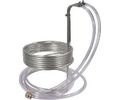
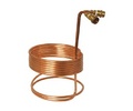
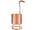
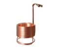
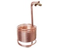
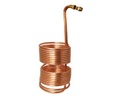
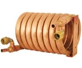
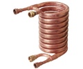
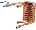
Counterflow wort chillers consist of two channels placed in physical contact with one another so that heat is exchanged between them. Various configurations are possible, but the design most familiar to home brewers is 25 ft of copper refrigeration tubing (usually ⅜ in., but sometimes ½ in.) inserted into a larger diameter garden hose, with suitable fittings at either end. Hot wort flows through the smaller diameter tubing inside, and cold water flows through the garden hose surrounding the tube so that heat transfers from the wort tube to the water. The coaxial tubes are nearly always arranged into a moderate diameter coil to make the unit easier to handle and store. In another common arrangement, the wort channel is again small-diameter (usually ⅜-in.) copper tubing, but wound into a small coil that is then inserted into a larger rigid PVC pipe, 4.5 in. or larger, through which the cooling water flows. Other designs are usually variations of these two and typically feature some means of enhancing the thermal contact between the two channels, such as fins attached to the inside tube, for example. In larger chillers for commercial brewing operations, the channels are often cut into stainless steel plates with the inlets and outlets arranged in such a way that multiple plates can be stacked, thus allowing a wide range of total channel lengths to be implemented. A chiller’s cooling capacity is directly proportional to the length of the channels. Doubling the length of a chiller of constant geometry thus doubles the amount of wort that can be chilled in a given time period. Regardless of the implementation, the wort flows through its channel in one direction and the coolant through its channel in the opposite direction. This means that the wort leaving the chiller contacts the coolant entering the system, where the coolant is coldest. For this reason, counterflow chillers ensure the greatest degree of cooling possible. |
Before delving into the question of how to determine the value of Q for our chillers, let’s first explore some applications of Q in our breweries. The examples in the following sections assume known values of Q.
Looking for a wort chiller? Click here to browse our selection of counterflow wort chillers!
A chiller’s effectiveness is defined in terms of efficiency, which would be 100% if the temperature of the wort leaving the chiller were exactly the same as the temperature of the coolant entering it (the 100% condition). It is impossible for the exiting wort to be cooler than the coolant, and for practical purposes 100% efficiency is unattainable, so efficiencies are generally somewhat less than 100% — how much less depends on the rates at which the hot wort and coolant flow past each other. The slower the wort flow, the faster the coolant flow, and the greater the thermal conductivity between wort and coolant, the greater the efficiency.
Determining the efficiency of any chiller setup is a simple matter. First, we must determine the potential temperature drop for wort flowing through the chiller, which is the difference between the temperature of the hot wort entering the system and the temperature of the coolant as it enters the system. The chiller’s efficiency is simply the fraction of this potential temperature drop that is actually realized. To calculate efficiency, take the difference between the entering and exiting wort temperatures (actual temperature drop) and divide that number by the potential temperature drop:
.jpg) [1]
[1]
where η (the Greek letter eta) is efficiency, Tw(0) is the temperature of the wort at its point of entry to the wort chiller, and Tw(L) and Tc(L) are the temperatures of the wort and coolant at the outlet (L represents the length of the chiller).
Suppose you know the efficiency values for your chiller when operating at given wort and coolant flow rates. It is now a simple matter to compute the temperature at the outlet of your chiller. First, determine the equivalent efficiency loss (1 minus its efficiency, where the efficiency is expressed as a decimal); this is the chiller’s potential cooling loss. Multiply this potential cooling loss by the potential drop to get the actual cooling loss (in degrees). Add the cooling loss to the coolant inlet temperature to get the wort output temperature. This relationship can be expressed with the following equation:
Tw(L) = Tc(L) + (1 – η) [Tw(0) – Tc (L)] [2]
For example, if a chiller uses 55 °F (~12.75 °C) cooling water with wort entering at 212 °F (100 °C), the potential temperature drop is 212 – 55 = 157 °F (87 °C). If it is operating at 98% efficiency, the lost potential is (1 – 0.98) X 157 = 3.14 °F (~1.75 °C), and the outlet temperature is 55 + 3.14 = 58.14 °F (~14.5 °C).
Understanding chiller efficiency is the key to understanding how to predict and control the variables of wort flow rate, coolant flow rate and consumption, and chill time.
Interested in an immersion wort chiller? Click here to browse our selection!
Chiller performance can be determined graphically, without the use of detailed calculations. Figure 1 displays curves of constant efficiency. The vertical axis (y-axis) is the flow rate of the wort, and the horizontal axis (x-axis) is the flow rate of the coolant. In both cases, the flow rates are normalized by Q; wort flow is further adjusted for specific gravity (ρ).
To use the graph, first multiply the wort flow rate by the wort’s specific gravity and divide by Q, and find that value on the vertical axis of Figure 1. Suppose, for example, your chiller has a Q of 68. If wort of specific gravity 1.050 flows through it at 34 gal/hour, the normalized flow is (34 X 1.050)/68 = 0.525. Thus, we look for the value 0.525 on the vertical axis.
Similarly, divide the coolant flow rate by Q and find that value on the horizontal axis. To continue the example, let’s assume our coolant flow rate is 240 gal/hour, which divided by 68 gives a normalized flow of 3.53. That’s the number we look for on the horizontal axis.
If we draw a horizontal line from 0.525 on the vertical axis and draw a vertical line from 3.53 on the horizontal axis, the lines intersect. The point of intersection reveals the efficiency of this particular chiller setup. These lines have been drawn in on Figure 1, and they intersect between 80% and 85%, but closer to 85%, from which we can estimate that the efficiency is about 83%. This compares well with the value of 82.8% obtained using formulas.
Each curve represents a constant efficiency. Any combination of normalized wort and coolant flows that falls on a particular curve will have the efficiency of that curve. For example, a normalized wort flow of 0.2 and a normalized coolant flow of 10 result in 99.326% efficiency, as does a normalized wort flow of 0.17 and a normalized coolant flow of 1.0. (Both of these points fall on the heavy curve of Figure 1.)
Using efficiency data to determine required flow rates: Brewers usually know how cold they want the output wort to be. With known hot wort and inlet coolant temperatures, you can quickly determine the efficiency you require to get there. Once you know the required efficiency, you can move along the curve for that efficiency and find nominalized flow rates for wort and coolant that meet your operating criteria. Understanding the relationships between efficiency and flow rates enables you to take dramatic strides in the control of wort chilling operations.
As an example, suppose you want to cool 212 °F wort to 52 °F (11 °C) using 50 °F (10 °C) cooling water. Assuming the wort enters the chiller at boiling, you need the following efficiency:
η = (212 – 52)/(212 – 50) = 0.9876, or 98.8%
Looking at the chart, the closest efficiency line is the 99% line, so you may choose any point along that line, such as a normalized wort flow of 0.14 and a normalized coolant flow of 0.3, or a normalized wort flow of a little over 0.2 and a normalized coolant flow of 10.
Comparing the two choices raises a couple of interesting observations about the graph. First, the first option results in a longer chilling time but a lower coolant flow rate; the second operating point gives a faster chilling time but requires a higher water flow rate. If you want quick chilling to minimize DMS formation in your beer, you would probably be inclined to select the second option. Second, we can see that all the curves roll over and become pretty flat at a normalized coolant flow rate of about 1. You can run the chiller at this value (a big difference from 10) and still have a normalized wort flow rate of 0.18 (a relatively little difference from 0.2).
The graph gives us a range of normalized values for wort and coolant flow rates, but how do we know the actual flow rates to use? Determining actual flow rates is a simple matter of working the calculations backwards and un-normalizing them.
Small chillers of the type usually purchased by home brewers generally have Qs around 65. Using that value with the three choices just offered, we can un-normalize (multiply the normalized flow by Q) and arrive at some real numbers (Table I). The times and coolant consumption values shown in Table I are based on a 10-gal batch (we chose this batch size because a chiller with a Q of 65 is really too small for larger batches).
To simplify the calculation, we can ignore the specific gravity factor in the wort flow rate. Neglecting this factor causes the calculated un-normalized wort flow rate to be bigger (by about 5% for S.G. 1.050) than it would be if specific gravity were taken into account, resulting in poorer chiller efficiency than calculated. Although this effect can usually be ignored, you should be aware of it and may wish to use the specific gravity factor in all calculations (or perhaps only those applied to dense worts).
The table shows that the slowest option is the most economical in terms of the amount of coolant water used, which is what one might suspect. The fastest option will cool the wort in two-thirds the time, but at a cost of 25 times the cooling water and a coolant flow rate that is not achievable with most home water supplies. The intermediate option requires about 2.5 times the cooling water of the slow option and reduces cooling time by 15 minutes. This middle ground seems the best choice, but in special circumstances as where, for example, DMS production is a big problem or water conservation is an important issue, brewers might prefer one of the other choices. This example demonstrates the value of these curves and formulas.
The rule of thumb: Note that the intermediate choice here also reveals an easy-to-remember rule of thumb for good performance: Where it is possible to establish wort flow at a rate of Q/5 or less, exiting wort will be chilled to within 3 °F (1.7 °C) of the available coolant temperature, as long as the cooling water flow is equal to or greater than Q. Mathematical (rather than graphical) computation of the efficiency for this rule-of-thumb operating point gives an efficiency of 98.53%. Applying equation 2 tells us that if the entering coolant temperature is 32 °F (0 °C) and the entering wort temperature 212 °F, wort exit temperature will be 2.6 °F (1.4 °C) above the entering coolant temperature, or 34.6 °F (1.4 °C). (This example shows the extremes of wort and coolant temperatures. The difference between exiting wort and entering cooling temperatures will be somewhat less when coolant temperatures are higher and wort temperatures are lower.) Because 3 °F is easier to remember than 2.6 °F, we usually speak of a less than 3 °F rise for the “Q by Q/5” operating point.* As we shall see shortly, it is not always possible to realize a wort flow of Q/5 because reducing the wort flow rate reduces Q. Sometimes lower levels of efficiency must be accepted.
|
Spreadsheet Examples |
|
The data from your temperature measurement experiments can be calculated in a simple spreadsheet program, like Excel (Microsoft, Bellevue, Washington). The example spreadsheets shown here are provided in two forms — one with data, and the other showing the formulas behind the data. Other spreadsheet programs will require similar formulas in the cells. Spreadsheet row and column identifiers (numbers and letters) are shown to help you correlate the numbers with the formulas that produced them. The first spreadsheet shows the experimental data set obtained from Chiller B. The first column has entries for the number of seconds required to fill a pitcher to the 1-L mark. The second column indicates the hot water inlet temperature. The third column contains the entries for the measured wort (in this experiment, boiled water) outlet temperature. The fourth column is the coolant inlet temperature. The fifth column contains wort flow rates computed from the times in the first column. The sixth column contains values for the coolant flow rate. The seventh column holds computed values for efficiency; the eighth, computed values for αL; and the last column contains the computed values of Q. Values for m and b obtained for the best linear fit to the pairs of Fw and Q are displayed in two labeled cells at the bottom of the spreadsheet. The formulas necessary to compute efficiency and Q are all given in the boxes on pp. 52–53. For clarity, the next spreadsheet shows the formulas actually used to compute the values in the previous spreadsheet. One peculiarity of Excel is that the LINEST function, used to estimate m and b, requires that two cells be dragged over to reserve space to display the two answers, the formula must then be typed in as indicated in the leftmost cell only, and then the command and enter keys must be pressed simultaneously to enter the formula. If this is not done, only the m value will be displayed. The next spreadsheet illustrates the calculation of an efficiency curve from the m and b numbers obtained using the first spreadsheet. In the second row (just below the labels) find values for the model parameters for Chiller B and the coolant flow rate (Fc). The wort flow numbers in the first column are all within the range specified for this chiller and were chosen to fill in the span with enough points to give a smooth curve and keep the spreadsheet size modest enough that it could be printed here without using too much space. Any other spacing can be used. The second column is values of Q computed from the model parameters for this chiller using equation 3. The third column contains computed values of αL computed from equation 11, in the fourth column this has been exponentiated, and in the final column are computed values of efficiency obtained from the formula of equation 12. (Note that these efficiency numbers are not the same as those plotted for Chiller B in Figure 4, because we chose to do these calculations with a coolant flow rate of 150 gal/hour rather than the 340 gal/hour used in doing the calculation for the figure.) The final spreadsheet displays the formulas, in Excel format, used in setting up the efficiency spreadsheet. |
Now that we know the importance and usefulness of Q in evaluating chiller performance, we need to know how to obtain values of Q for our own chillers. Some values have been published, but what we need is a means of measuring the values for our own chillers.
The exercise required to determine Q for your chiller is simply a matter of heating some water to boiling, running it through the chiller, measuring the inlet and outlet temperatures and the wort and coolant flow rates, and calculating the chiller’s efficiencies at various flow rates. Finally, those values will be processed to determine Q, either with the help of a spreadsheet, a calculator or Figure 1.
![]() *Wort temperature may exceed 212 °F by 1–2 °F, especially if the wort is of high gravity. Using 3 °F rather than 2.6 °F in the specification of maximum rise more than makes up for this added variable.
*Wort temperature may exceed 212 °F by 1–2 °F, especially if the wort is of high gravity. Using 3 °F rather than 2.6 °F in the specification of maximum rise more than makes up for this added variable.
|
Table I: Cooling Time and Coolant Used to Chill Wort at Various Flow Rates for a Q of 65 |
|||||
|
Normalized (gal/hour) |
Un-normalized (gal/hour) |
||||
|
Wort Flow |
Coolant Flow |
Wort Flow |
Coolant Flow |
Time for 10 Gal (min) |
Coolant Used (gal) |
|
0.14 |
0.3 |
9.1 |
19.5 |
66 |
21 |
|
0.18 |
1 |
11.7 |
65 |
51 |
56 |
|
0.20 |
10 |
13.0 |
650 |
46 |
500 |
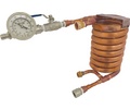
Determining efficiency values: Measure wort temperatures. Be sure to measure the wort temperatures just where the wort enters and leaves the chiller. Some chillers come with a thermometer installed in a compression “T” right at the outlet. Installing another one of these at the inlet is ideal. If no thermometer was supplied with your chiller, try piercing a small hole in the plastic wort tubing where it joins the chiller. Then insert a dial-type thermometer through the small hole in the plastic tubing with the probe along the axis of the tubing and the tip right where the wort enters/leaves the chiller. If the hole in the tubing is small enough and the fit tight enough, any leakage from the installation should be small. Some sort of sealing compound could probably be used to make the pierce point water-tight. Be sure that all thermometers have been calibrated.
Measure coolant temperature and flow rate. Turn on the cooling water full blast, and allow a few minutes for the cooling water temperature to stabilize and to ensure that the temperature is that of the well or city main and not that of the pipes in your house or brewery. Measure the flow rate by timing how long it takes to fill a container of known capacity (a 1-gal jug, for example). Getting a good measurement here could be a bit tricky because the flow rate may be high enough force water out of the exhaust hose with some violence.
Measure wort flow rate. Now allow the “wort” (boiling water) to flow from the kettle through the chiller. Get a wort flow measurement by timing how long it takes to fill an accurately calibrated container to a given mark (1 L or 1 qt is a good amount for a small chiller). The time taken for the flow measurement should be sufficient for the temperature readings to stabilize, but check to make sure that they are stable. When you are certain, record inlet and outlet temperatures.
Take a range of readings. As soon as you have a measurement pair, reduce the wort flow (by closing a valve or tightening a ‘C’ clamp onto a hose, for example) and repeat to obtain a series of measurements. The measurement set should include a slow-end wort flow with outlet temperatures within half a degree or so of the coolant temperature. The fastest flow should be as fast as the system can supply wort to the chiller.
A small pump can help you control wort flow rate and get a good range of wort flow rates and a uniform flow rate. If you use a pump, be very careful, because flow control is best achieved by throttling at the output, which pressurizes the line between the pump and the throttling device. The plastic hoses often used by home brewers become soft at boiling temperatures and can pop off their barbs unless tightly clamped, resulting in boiling water sprayed around the setup area.
Calculate efficiency. For each set of measurements calculate the efficiency using equation 1. If you wish to determine Q graphically, multiply by 100 to get a percent value; if you plan to use the formulas given at the end of the article, leave values in decimal form.
Calculating Q: Now calculate values for Q from your data pairs. This is best done using a spreadsheet (an example spreadsheet is shown in the box, “Spreadsheet Examples”), with a calculator using the equations developed later in this article (see box, “Mathematical Formulas for Q”), or graphically (using Figure 1). Although the calculations give the most accurate results, examining how this can be done graphically illustrates an important point.
Example. In one experiment, hot water flowing at 53 gal/hour was cooled from 212 °F to 61 °F (16 °C). The cooling water was at 56.5 °F (13.6 °C) with a flow rate of 290 gal/hour. These numbers give an efficiency of 0.9711 or 97.11%.
To solve for Q graphically, divide the wort flow rate by the coolant flow rate. In the example, the ratio is 53/290 = 0.1827. Next, go to the performance graph (Figure 1) and find the vertical line representing 0.1 normalized coolant flow. Move up the line until you find the value on the vertical axis that corresponds to 0.1 times the ratio of the flow rates or 0.01827 in this case. Make a mark at that point. Now go to normalized coolant flow 1.0 and move up its vertical line to 0.1827 and mark that spot. Draw a straight line between the two marks (see Figure 1). Note that any points representing the flow ratio can be used, such as (0.2, 0.03654), (0.3, 0.05481), (4, 0.7308), etc. to facilitate the drawing of the straight line.
The straight line should pass through the family of efficiency curves away from the part of the graph where they are bunched up (see Figure 1). If your straight line does not do this it is because the ratio of wort flow to coolant flow for this measurement was too high. Note this, and regard the Q value determined from this temperature pair with suspicion. Such values of Q are known to be inaccurate whether determined from a graph or by the formulas. Q is said to be “poorly observable” under these conditions.
Next, find the point at which the straight line just drawn intersects the measured efficiency curve. In our example, the efficiency was 97.11%. Because the graph shows no curve with that value, we must interpolate between the 97% and 98% curves. 97.11% is much closer to 97% than to 98%, so we try to visualize where the straight line would cross a curve parallel to the 97% curve and about one-tenth of the distance to the 98% curve. Read the value of this intersection from either axis. It appears to be at a level of about 0.26 on the wort flow axis and about 1.4 on the coolant flow axis.
Finally, take these normalized values and divide them into the actual flow rates to get estimates of Q. Dividing 0.26 into the wort flow of 53 gal/hour gives Q = 204, and dividing 1.4 into the coolant flow of 290 gal/hour gives Q = 207 as estimates for this chiller. These results are consistent within the limits of what can be expected from reading graphs and compare favorably with the value obtained from formulas (217).
Multiple readings and the straight-line fit: Determine values of Q from your other temperature data pairs and then plot them against the “wort” flow rate.
Figure 2 shows an example of what the plot might look like. These data were taken from experiments with a commercially available chiller (called Chiller A here). The chiller has a coaxial design, consisting of a 0.5-in. o.d., 0.39-in. i.d. copper tube enclosed in a 0.93-in. o.d. steel tube formed into a 5-in. (average) diameter coil of 4.5 turns. Thus, the length of the chiller if straightened out would be about 6 feet. The measured values of Q are indicated by open circles. They were obtained in two separate experiments with coolant flow of 170 gal/hour for some and 230 gal/hour for others. (Note that the determined value of Q is insensitive to changes in coolant flow rate of this magnitude. Nevertheless, some of the variation in the measurements is due to this factor; other factors include errors in flow rate measurement and thermometer reading.)
Figure 2 makes it clear that Q increases linearly with increasing wort flow rate. In keeping with common practice, I drew a straight line that best fits the data. For your data set, you can use the linear regression capabilities of your spreadsheet program to obtain this line (the example spreadsheet in the box on pages 46–47 shows how to do this with Excel), or draw it on the data plot with a ruler.
Why does Q vary with wort flow rate? At higher wort flow rates, the flow in the inner tube is more turbulent, which allows more of the total volume of the wort to contact the cool outer wall of the wort tube. This accomplishes better thermal transfer from the wort to the tube wall. This increase, however, does not continue forever. When the flow becomes totally turbulent,* Q will not increase further with increased wort flow. One may well ask whether the same principal applies in the coolant channel. It does, but we are ignoring that for this analysis because the coolant flow rates are much higher than the wort flow rates in the usual application (that is, we assume the coolant flow to be fully turbulent).
Rather than deal with the set of individual measurements as represented by the circles on the figure (our original intent was to come up with a single number that describes a chiller’s Q value), we characterize the chiller by the straight line fit. This is feasible because the measured data are well described by a straight line, and it is desirable because a straight line can be described by two numbers, m (slope) and b (intercept). Your spreadsheet can easily generate a straight line, and the slope and y-intercept, using a regression routine.
In preparing this article, I made measurements on two other commercially available chillers as well. The first is a small unit fabricated from about 25 ft of ⅜-in. refrigeration tubing formed into a coil and placed inside a piece of 5-in. PVC pipe. The other consists of 50 ft of ½-in. refrigeration tubing coaxial with a 1-in. i.d. rubber hose formed into an 11-turn coil about 16-in. in diameter. Both units were measured with coolant flow rates of about 340 gal/hour, and each yielded a set of data points that were well fit with a straight line. These straight line fits are plotted in Figure 3, together with the fit from the first chiller so that all three can be compared.
Table II gives the number pairs (m,b) for all the chillers measured. While the table gives no information beyond what is given in the graph, it provides numerical information that can be used to reconstruct the graph with the following formula:
Q = mFw + b [3]
where Fw is a wort flow rate between the minimum and maximum values determined for the particular chiller, and m and b are the slope and intercept values for the chiller, m and b are provided by the linear regression tools in your spreadsheet program. You can do it by hand by using your best fit curve through the data points: m = (change in Q)/(change in Fw); b = the value of Q at which the extended fit line crosses the Q (vertical) axis.
For example, if we operate Chiller A at a flow rate of 50 gal/hour, Q = (1.1936 X 50) + 101.15, or 160.83; that number compares well with the value shown for 50 gal/hour wort flow rate in Figure 2. If we operate that same chiller at a wort flow rate of 30 gal/hour, then Q = (1.1936 X 30) + 101.15, or 137, which also fits the line in Figure 2.
The limits and the values for m and b constitute a “mathematical model” of the chiller. This model provides a concise means for specifying the relative performance of a set of chillers, taking into account variations in Q with wort flow rate. It can also be used to predict the performance of particular chillers. This is simply an extension of the methods already introduced for single values of Q.
It is hoped that Table II will be enlarged by this writer as well as other investigators to the point where enough data is available to brewers to allow them to chose the best chiller for their needs.
Confronted with data like those in Figure 3 (or Table II), how do you make decisions as to whether a particular chiller is suitable for your needs? You can find the answer by converting the mathematical model of the chiller into an efficiency curve using mathematical formulas (see box, “Mathematical Formulas for Efficiency”). This is also best done with a spreadsheet program, but it is also possible to use Figure 1 or a calculator.
First, pick a convenient number of wort flow values within the range of wort flows specified in the table for the chiller of interest. Enter these into a column of the spreadsheet.
|
Table II: Chiller Performance Parameters |
||||
|
|
Parameters |
Applicable Flow Range (gal/hour) |
||
|
Chiller |
m |
b |
Minimum Fw |
Maximum Fw |
|
A |
1.1936 |
101.15 |
24 |
110 |
|
B |
1.6521 |
19.83 |
1 |
44 |
|
C |
3.4481 |
21.575 |
5 |
115 |
Next, use Q = mFw + b in another column of the spreadsheet to calculate values of Q corresponding to the chosen values of wort flow.
Then calculate values of αL for each value of Q using equation 11 (see box, “Mathematical Formulas for Efficiency”). Use the values for the coolant flow you intend to use in actual operation in this equation. You may use a value other than 1 for wort specific gravity if desired.
Next, calculate values of efficiency from equation 12 (see box). This and the previous step can be skipped, and efficiency for each value of Q can be determined from Figure 1 using the method given previously.
Finally, plot the efficiency against the wort flow.
The calculations for the three chillers we measured are plotted in Figure 4. These data are for a wort specific gravity of 1.000. Coolant flow of 230 gal/hour was used for Chiller A and 340 gal/hour for Chillers B and C.
If you made measurements on your own chiller, you could simply plot the efficiencies you measured against the wort flow rates for which you obtained them and obtain a plot similar to that in Figure 4. This is adequate for most purposes, but I would nevertheless encourage you to go through the calculations and linear fit so that you have the data from which a comparison to other chillers can be made. The mathematical model also allows efficiency to be calculated for coolant flows other than that at which the measurements were taken.
Figure 4 allows you to determine the performance of any of the plotted chillers vis à vis your requirements. A couple of examples illustrate the usefulness of method:
Example 1: You want to cool 10 gal of boiling wort to 55 °F as fast as possible (to minimize DMS formation) using cooling water at 50 °F. The allowable rise of 5 °F with respect to a cooling potential of (212 – 50) = 162 translates to a required efficiency of 97%. Figure 4 shows that Chiller B is capable of delivering this level of efficiency at a wort flow of 10 gal/hour; cooling your 10 gallons of wort would require 1 hour. Chiller A will deliver the same efficiency at 36.5 gal/hour and would require about 16 minutes. Chiller C will do the job at 47 gal/hour in 13 minutes.
Example 2: A pilot brewery has a 2-bbl (62-gal) system and wants to chill within 1 hour. What outlet temperature can they expect if the coolant is at 50 °F? Chiller A, at a flow rate of 62 gal/hour, is capable of 90.5% efficiency or an efficiency loss of 9.5% The rise over the coolant temperature is thus 0.095 X 162 = 15.4; the output temperature would be 65.4 °F. Chiller C can deliver 96.4% efficiency for an efficiency loss of 3.6%; this means a rise of 0.036 X 162 = 5.8 for an output temperature of 55.8 °F.
|
Mathematical Formulas for Efficiency |
|
Per unit length, the amount of heat that flows between the wort and cooling water during a unit of time at any point along the length of the chiller depends on the difference in temperature between the wort and the coolant, the area (per unit length) in thermal contact and the thermal conductance between the channels. The heat lost by the wort is gained by the coolant. The temperature drop due to loss of a unit of heat is inversely proportional to the thermal mass (actual mass times a constant called the specific heat) of the wort, and the temperature rise of the coolant is inversely proportional to the thermal mass of coolant which pass the point in the unit time. Therefore, the temperature change of each of the fluids passing this point on the chiller is inversely proportional to the flow rate of the fluid. We want the wort temperature to change as much as possible and the coolant temperature to change as little as possible (so that it stays cold throughout the length of the chiller, thus maximizing the temperature difference at each point). Clearly, then, very high flow rates for the coolant and a very low flow rate for the wort are desirable conditions. These facts allow us to write two linear differential equations, one for the rate of change of temperature of the wort as it moves along the chiller, and one for the coolant. For our present purpose, it is sufficient to give the combined solution (e-mail the author for details):
Equation 4 expresses the efficiency of the chiller in terms of its length, L, and the new parameters α, kc, and kw. The first is simply the difference of the other two: α = kw –kc [5] and so it is kc and kw that determine the efficiency of the chiller. These parameters contain the information about the geometry, conductance, specific heat, density and flow rates. For the wort:
where W is the contact area per unit length, G is the thermal conductance per unit length, Fw is the wort flow rate per unit time, dw is the density of the wort, and Sw is the specific heat of the wort. Similarly for the coolant we have:
where W and G are the same because they describe the common interface between the two channels, but the other parameters are distinct because wort has different properties than water. Looking back to equation 4, we can see that the k’s appear in sums and quotients. Looking at the differences first we see that the exponent is
We can simplify things a lot if we assume that the specific heats of water and wort are about the same and note that the ratio of their densities is simply the specific gravity of the wort which we symbolize by the Greek letter rho, ρ. This gives
What we have done here is to separate all the things we do know about (flow rates, specific gravity) from the things we are not so sure about (internal geometry, conductivity and even the exact length of the channel), all of which we put into the factor which we call Q. Its definition is thus:
and so we now have:
When we take the ratio of the k’s, things cancel out under the same assumptions we used for the difference, and we get:
Given a value of Q, the flow rates and the specific gravity of the wort, all of which can be measured, we can calculate efficiency. Defined this way, Q is proportional to the thermal conductance per unit area between the channels. In this derivation, we assume that we have a value independent of wort and coolant flow rates. The validity of this assumption depends on the flow rates through both channels being high enough that the flows are turbulent. If either flow rate drops below the value required for turbulent flow, the thermal conductance between the channels drops, as does Q. It is easy to see why this is so. If the wort flow, for example, is smooth, heat at the center of the wort tube has to pass radially through the wort that is closer to the tube wall to reach it. The wort itself is not a very good conductor of heat. If, on the other hand, the wort is tumbling and mixing as it flows through the tube, all of it has an equally good chance of coming into contact with the cool tube wall. The measured data of Figure 2 clearly show that there is a dependence on the wort flow rate, and the significance of this fact has been discussed. As an example of the calculation of efficiency consider a chiller that has a Q of 68 with 34 gal/hour flow of 1.050 wort and a coolant flow of 240 gal/hour. Use of these numbers in equation 11 gives αL = 1.6328, and using that in turn in equation 12 gives η = 0.8277. |
You can use the efficiency curve for your chiller to select the operating point (wort and coolant flow rates) that best meets your requirements, but the values you actually wind up using will probably be determined for you to some extent. You will probably hook up your coolant line to a garden hose bib and turn on the water. In most homes, this will result in a flow of 200–350 gal/hour. This is clearly more than is needed for a small chiller.
Should anything be done about this? The answer depends on how you feel about water use. My water does not come through a water meter but rather from a well that has good flow year round. Uses can often be found for the coolant water. In the summertime, for example, I use it to water the garden. Other times, I allow it to flow back onto the ground outside where some of it, presumably, eventually makes its way back into the well. In continuous brewing operations, the wort chiller can be used to warm the incoming main’s water, which is to be used in mashing and sparging; the brewery thus recovers some of the heat energy that otherwise would be lost.
Where water use is restricted, more careful management is required. Obviously the supply valve can be partially closed but the question then becomes one of making sure that the flow rate is adequate and reasonably accurate. The gadget buffs can, of course, buy flow meters, with the ultimate measure of success being an output wort temperature close to that desired.
The most conserving approach to cooling water is to fill a pot with water and ice and to circulate this ice water through the coolant channel of the chiller with a pump (see Bennett Dawson’s article, “An Ice Water Wort Chiller,” in a recent issue of BrewingTechniques [3]). Flow rates can be measured in the same ways as suggested in this article. Use 32° F as the temperature of the coolant in calculations, but be aware that this temperature is maintained only if the water has a lot of ice in it. In this arrangement you are using the heat of the wort to melt ice and you may be surprised at how much ice is required (about 8.3 pounds for each gallon cooled from boiling to 68 °F). Be sure you have enough on hand.
In the typical home brewing setup, the wort passes through the chiller under the force of gravity. This means that the flow rate depends on how much above the chiller the surface of the wort is. As the wort is drawn off through the chiller, its level falls and so does the flow rate. A slow flow rates mean better chilling (see Figure 4); this is usually not a problem unless you are concerned that the extra time will result in extra cooling water consumption. Conversely, as Figure 4 also shows, increased wort flow rates can reduce cooling efficiency sharply, especially if the chiller is small. Better control and therefore uniformity of flow rate can be achieved by the use of a wort pump.
All contents copyright 2024 by MoreFlavor Inc. All rights reserved. No part of this document or the related files may be reproduced or transmitted in any form, by any means (electronic, photocopying, recording, or otherwise) without the prior written permission of the publisher.


.png)
.png)
(1).png)
.png)


.jpg) [4]
[4].jpg) [6]
[6].jpg) [7]
[7].jpg) [8]
[8].jpg) [9]
[9] [10]
[10] [11]
[11] [12]
[12]